Vectors and Matrices

Matrices and Vectors

MathCAD makes extensive use of matrices and vectors. A vector is defined here as a single column matrix. Matrices can be created by manually entering data, reading data from a text file, or cutting and pasting from another program such as Excel. To manually enter a matrix, select the insert matrix button from the matrix palette. Fill in the number of rows and columns desired in the resulting dialog and press enter. Place the cursor on the first place holder, enter the first value. Press tab to proceed to the next.placeholder and so on.

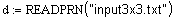
Entering a matrix manually is fine if you have small amounts of data. However, it is quite inefficient if you are entering hundreds of pieces of data, such as from a data acquisition system. MathCAD provides the function READPRN( ) to read data from an ASCII file. The argument to this function is a string, placed in quotes, representing the file name. The data file containing the matrix data is a pure text file typed in the same format as the matrix you want to display. The text file must be a pure ASCII file. That is, is is best generated by using a text editor such as NotePad. If you use a word processor, a spreadsheet or some other program to generate the file, make sure you use the 'Save As' feature to save the file as an .txt file.

<= Read Matrices

<= Display Matrices

NOTE: MathCAD also includes the function READ( ). This function is obsolete and should not be used. It is provided for backward computability only. Future versions of MathCAD may not include READ( ) function so its use is highly discouraged.

NOTE: MathCAD also includes thirteen other variations of the read function including READ_IMAGE, READ_BLUE, READ_HLS, etc. These are specialized functions used to read numeric data from raster images such as BMP, JPEG, GIF, TGA, and PCX. These functions will generate a matrix of data values representing that image. These functions are not covered in this course. To find out more, type 'READ' into the Index tab of the help dialog.

MathCAD also allows the results of matrix manipulation be output for further analysis or use by other programs. To do so, use the function WRITEPRN( ).

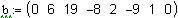
<= Dot product of matrices 'a' and 'b'

<= Display the result

<= Write results to file. If the file does not exist, writeprn( ) will create the file. If the file already exists, the current file will be overwritten. Use Notepad to view the file now.

If you need to append data to an existing file, use the APPENDPRN( ) function. This <= function will NOT create a file if it does not exist.

NOTE: Both functions will be invoked when you enter them initially. If you need to invoke them again, place the cursor on the function and recalculate by pressing F9 or selecting 'Calculate' from the Math menu item.

Be cautious when recalculating the APPENDPRN( ) function. This function will continue to append data to the specified file resulting in a very large matrix with redundant data.

NOTE: MathCAD also includes the functions WRITE( ) and APPEND( ). These functions are obsolete and should not be used. They are provided for backward computability only. Future versions of MathCAD may not include either function, so their use is highly discouraged.

Once an array is entered and manipulated, we must have some way to extract the data from any given array. All elements of vectors and arrays are addressed through subscripts. An array subscript is entered using the left square bracket ( [ ) key. By default, all vectors and arrays are indexed such that the first row and column are row and column zero. Thus the first element of any matrix 'M' is M_0,0.

Addressing elements of a vector

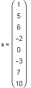
Display vector 'a' from above =>

<= You cannot use the literal subscript as entered with the period key, to address a matrix item.

<= Enter an array subscript using the square bracket key. In this case, use the keystrokes a [ 1 =

<= Sometimes, you may want to change the origin of a matrix to something else. Do this by going to the Math, Options menu. If changing this value within the dialogue, it will affect the entire worksheet. Alternatively, you the variable ORIGIN can be addressed and changed from within the worksheet as shown. If you change the array origin this way, it affects only the area of your worksheet below the declaration.

<= With the origin set to one, the first element of vector 'a' is now a₁. Element a₀ no longer exists.

<= Reset origin for remainder of lecture

Addressing elements of a matrix

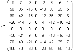
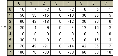
<= Display matrix 'c' as calculated above

The element of matrix 'c' occupying the zeroeth row and zeroeth column

The element of matrix 'c' occupying the seventh row and seventh column

With ORIGIN set to zero, the last row of matrix 'c' is the seventh row, not the eighth There is no row eight so this designation is an error

There are also situations when we may need to extract entire rows, columns or submatrices of data from a matrix To do so, we can use the M^<> function (from the matrix palette) and the submatrix( ) function.

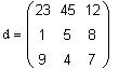
<= Read a matrix from a file

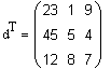
<= display matrix

<= extract the second column (this is column 1 since the array origin is set to zero). Use M^<> (ctl-6) to do so.

<= To extract a row, we must first transpose the matrix using the M^T (ctl-1) function from the matrix palette

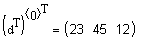
<= If we want row zero of the original matrix, we would extract column zero of the transposed matrix. Note the functions are nested.

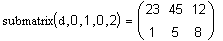
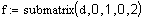
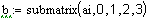
<= We can also extract an entire submatrix using the function submatrix(M,r1,r2,c1,c2). The function shown to the left generates a matrix comprised of rows zero and one from the original matrix 'd'. Note we can either declare it for purposes of display or assign it to a variable for later use.

There are many instances where we need change the size of a matrix. In this case, this means adding individual rows and/or columns at random points throughout an existing matrix. This can also mean augmenting or stacking two or more existing matrices.

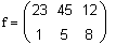
<= Create matrix 'f'

<= To add a column, place the cursor on the column immediately to the left of the column you want to add. Press CTL-M. In the resulting dialog, enter zero rows and one column. Click on insert. A column will be inserted to the right of your cursor.

<= Similarly, you can add a row by placing the cursor on the row immediately above the row you want to add. Press CTL-M. In the resulting dialog, enter 1 row and zero columns. Click on 'Insert'. A row will be inserted immediately below your cursor.

Deleting a row or column is similar. Simply place the cursor on the row and/or column you want to delete. Press CTL-M. In the resulting dialog, enter the number of rows and/or columns you want to delete. The specified number of rows/columns immediately to the right and below the cursor, including the row/column the cursor is in, will be deleted.

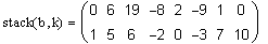
If you have two or more matrices, you may be able to stack or augment them. Creating a matrix using Stack(a,b ) means you will 'stack' matrix 'a' on top of matrix 'b' . As such, the matrices MUST have the same number of columns to be stacked. They may have a different number of rows.

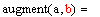
Similarly, to create a matrix using augment(a,b) means the matrix 'a' and matrix 'b' will be placed side by side to create a new matrix. As such, the matrices must have the same number of rows. They may have a different number of columns.

<= Display matrices 'a' and 'b' as read from file above.

<= Since matrix 'a' has 8 rows and matrix 'b' has only one row, they cannot be augmented. Likewise, the different number of columns in each does not allow them to be stacked.

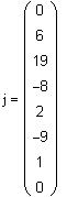
<= create matrix 'c' by transposing matrix 'b'
create matrix 'd' by transposing matrix 'a'

<= Display matrices 'j' and 'k'.

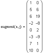
<= Since matrices 'a' and 'j' now have the same number of rows, we can augment them.

<= Similarly, matrices 'b' and 'k' have the same number of columns and can be stacked.

Most of the preceding functions are used to manipulate the appearance and order of the matrix or vector. Now we need to look at some matrix functions we can use for purposes of calculation and analysis.

<= Display matrix 'd' as calculated above

<= The functions shown to the left access the array to determine various properties of the array. The min( ) and max( ) functions find the numerical minimum and maximum values contained within the matrix.

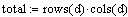
The row( ) and cols( ) functions determine the number of rows and columns that make up the matrix. Note the product would be the number of elements within the matrix.

All of these functions are valid for matrices and vectors.

<= The functions length( ), last( ) and S( ) (vector sum) are valid only for vectors. Length determines the number of elements in the vector while last returns the index value of the last element contained within the vector. Applying these functions to a matrix will result in an error.

Note we can nest the column extraction function with any of the vector functions to 'simulate a vector and perform the appropriate operation.

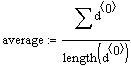
<= Note that one application of these matrix functions is statistics. For example, we can take the vector sum of the zeroeth column of matrix 'd' and divide that by the length of the zeroeth column of matrix 'd' to determine the average of that column of numbers.

Another matrix useful matrix function is being able to sort the elements of an array based on some criteria. The MathCAD functions available to do this are sort( ), reverse( ), csort( ) and rsort( ). The first two are applicable to vectors only. The last two are for multiple column arrays.

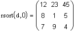
<= Display matrix 'd' as calculated above

<= Since the sort function applies to vectors only, we will generate a vector by extracting a column from matrix 'd'.

<= The sort function sorts the elements of vector 'e' from low to high

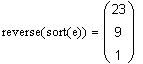
<= If you wish to sort the vector from high to low, apply the reverse function as shown.

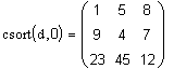
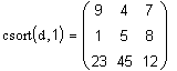
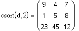
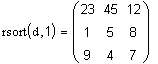
We can also sort the elements of matrix 'd' using the csort(v,n ) and rsort(v,n ) functions, column sort and row sort respectively. The arguments of these functions are vector ' v ' and the column or row 'n' upon which the sort is based. For example:

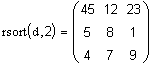
In the three examples shown to the left, we will sort matrix 'd' by columns 0, 1 and 2 respectively.

The first function resorts matrix 'd' by arranging column zero from low to high. The remaining elements of each row maintain their relative position.

The second function sorts matrix 'd' by arranging column one from low to high. The remaining elements of each row maintain their relative position.

The third function sorts matrix 'd' by arranging column two from low to high. The remaining elements of each row maintain their relative position.

The rsort( ) function does the same thing except by row. Examination of the three examples to the left show matrix 'd' sorted by rows zero, one and two respectively.

A common use of matrices is in the solution of simultaneous equations. To that end, we need to be able to invert a matrix. The inverse of any matrix 'a' is matrix 'b' such that the dot product of a and b will yield an identity matrix.

Example: Find the inverse of Matrix 'a'

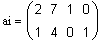
<= The first step is to augment matrix 'a' with an identity matrix. MathCAD provides the identity( ) function to allow easy creation of an identity matrix.

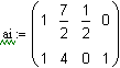
<= Create matrix 'ai' by augmenting matrix 'a' and ' I '.

<= Now perform a series of row operations such that the left half of matrix 'ai' is replaced by an identity matrix and the right half is replaced by the inverse. After performing these operations, you should end up with the matrix shown to the left

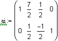
<= First, force the first element of matrix 'ai' to a value of one by multiplying row 1 of matrix 'ai' by 1/2.

<= Next, force the first element of the second row to zero by multiplying the second row through by the expression -1R₁ + R₂ where R₁ and R₂ are elements of the first and second rows of the matrix.

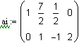
<= Next, force the second element of the second row to one by multiplying the second row through by 2.

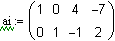
<= Finally, force the second element of the first row to zero using the expression -7/2R₁ + R₂ where R₁ and R₂ are the first and second rows of the matrix

<= Use the submatrix function to extract the right half of matrix 'ai'. This will be the inverse of matrix 'a'

<= Check your work by taking the dot product of matrices 'a' and 'b'. This should yield an identity matrix.

Of course, MathCAD allows us to do this same thing much easier by using the inverse function from the matrix palette.

MathCAD also allows one to calculate the determinant of a matrix.. The determinant of a matrix can be used to solve simultaneous equations (Cramer's Rule). It is also used to determine whether or not a system of simultaneous linear equations has a unique solution. A non-zero determinant indicates there is a unique solution. The matrix function can be selected from the matrix palette or entered by pressing the '|' key. Although MathCAD will calculate a determinate for any order matrix, the determinant is most useful when one has a square matrix.

<= The determinant of Matrix 'a'

An example of using the determinant and the inverse of a matrix is to solve simultaneous equations.

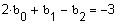
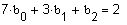
Find the solution to the following set of equations using matrix methods

Side Note:

The equations to the left are displayed with a bolded equal sign. This is a boolean equals. We will discuss this in a later lecture. For now, I use it strictly for display purposes. So as not to cause a calculational problem, these equations have been 'disabled' as indicated by the raised black square.

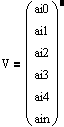
Define the coefficient,variable and solution matrices

First, let's determine whether or not this system of equations has a unique solution. To do so, we will find the determinant of the coefficient matrix.

Since the determinant is nonzero, this system of equations does have a unique solution. In matrix form, this system of equations is written as a*b=c. We can determine the contents of matrix 'b', the solution matrix, by multiplying both sides of the equation by the inverse of matrix 'a'

Since a * a^-1 is an identity matrix, the solution matrix 'b' is found simply by multiplying matrix 'c' by the inverse of matrix 'a'

Verify the correctness of this solution matrix by writing out each function as follows:

Another method is to use MathCAD's lsolve( ) function

Dot product vs. cross product vs. vectorize

The dot product refers to matrix multiplication. As with most matrix operations, it is an intensive

process when accomplished by hand. Unlike scalar multiplication, the dot product of matrices is not

commutative. In other words, V*U is not equal to U*V. A dot product can only be taken if the

number of columns in the first matrix equals the number of rows in the second matrix. In other

words, V_mxn*U_nxp is valid since matrix V has n columns and matrix U has n rows. The resulting

matrix will have m rows and p columns. However, U_nxp*V_mxn is not a valid dot product since matrix

U has p columns and matrix V has m columns.

The dot product of two matrices is defined as follows:

<= Display matrices 'a', 'b', and 'c' as defined above

For example, the dot product of matrix 'a' and 'b' will be a three row by one column vector. The

first element is the product of row zero of matrix 'a' and column '0' of matrix 'b'. It is calculated

as (1*-1)+(0*2)+(7*3) = 20. The second element is the product of row one of matrix 'a' and

column zero of matrix 'b'. It is calculated as (2*-1)+(1*2)+(-1*3) = -3. The final element is found

by multiplying row two of matrix 'a' and column zero of matrix 'b'. It is calculated as

(7*-1)+(3*2)+(1*3) = 2. MathCAD makes this easier with the dot product function selectable

from the matrix palette or entered using the asterisk (shift-8) key.

The examples shown to the left represent a variety of dot products of the three matrices 'a', 'b' and 'c'. Why is the dot product of b*a and c*a invalid compared to the dot products of a*b and a*c?

Why are the dot products of b*c and c*b both valid? Why are they equal?

Although a number of analysis methods require true matrix multiplication, there are cases where we would rather perform an element by element multiplication. MathCAD allows us to do this by using the vectorize function (CTL - -).

An element by element multiplication obviously yields a 3x1 vector with elements -20, -6 and 6.

<= Use MathCAD's vectorize function, as shown to the left, will perform this calculation for you.

A final matrix function is the cross product function. A cross product can be taken only with vectors consisting of three elements. The elements of these vectors represent coordinates in space, thus a direction and magnitude of the vector. The cross product of two vectors is given by c=a*b*sin(a) where a is the angle between vectors a and b. This concept is used significantly in statics to solve for forces on a structure. It is also used extensively in electronics.

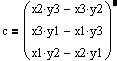
<= Assume vectors 'x' and 'y' as shown. The cross product of these vectors is some vector 'c' such that the elements of vector 'c' are defined as:

<= Display vectors 'b' and 'c' as previously calculated

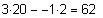
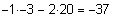
<= The cross product b x c is calculated by MathCAD as shown. The element by element derivation is shown below.

<= Note the cross product c x b is the cross product of b x c multiplied by -1.